
Sponsored Ads
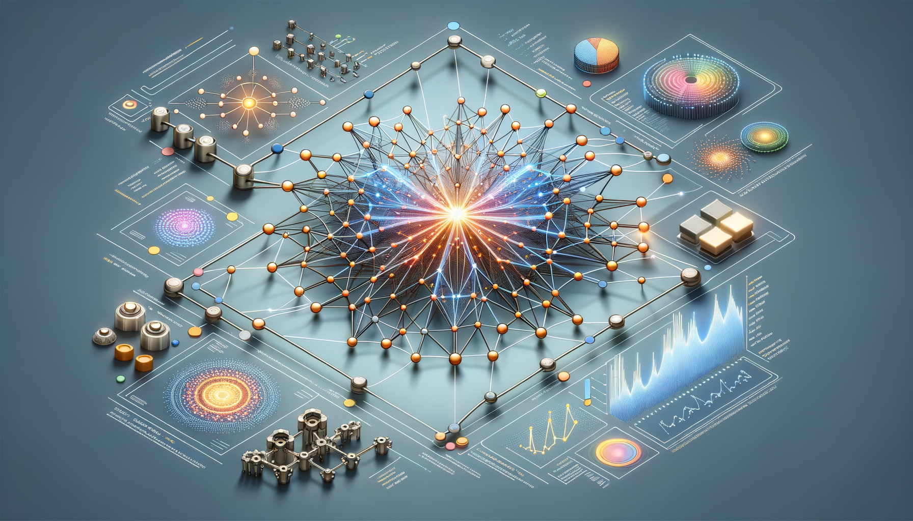
The hard truth many teams face today is that their data is deeply connected, but their models are not. Traditional machine learning treats records as independent rows, ignoring relationships like who follows whom, how items co-occur, or which molecules bind. Graph Neural Networks (GNNs) change that. By learning directly from nodes and edges, Graph Neural Networks (GNNs) turn relationships into signal—boosting accuracy in recommendation, fraud detection, drug discovery, knowledge graphs, and more. If your most valuable information hides in connections, this guide explains how GNNs work, where they shine, and the trends shaping what comes next.

In simple terms, GNNs extend deep learning to graph-shaped data. They aggregate information from a node’s neighbors, pass messages along edges, and stack layers to capture multi-hop structure. The result: embeddings that reflect both features and context. This article breaks down practical use cases, core architectures, and step-by-step guidance so you can build, evaluate, and deploy GNNs with confidence.
What Are Graph Neural Networks and Why They Matter Now
GNNs are a family of models designed to learn from graph data: sets of nodes (entities) connected by edges (relationships). Unlike CNNs for images or Transformers for text, GNNs operate via message passing. Each layer updates a node’s representation by aggregating signals from its neighbors, optionally weighting by edge types or attention scores. Over multiple layers, a node’s embedding captures wider relational context—friends of friends, co-purchase networks several hops away, or functional groups within a molecule.
Why now? Three converging factors make GNNs especially relevant: data reality, tooling, and scale. First, most high-value data is relational: social networks, transaction networks, product-user interactions, protein–protein interactions, road networks, and knowledge graphs. Second, modern libraries like PyTorch Geometric (PyG) and Deep Graph Library (DGL) have made GNN modeling approachable with efficient sampling and batching. Third, scalable training methods (neighbor sampling, graph partitioning) and public benchmarks like the Open Graph Benchmark (OGB) enable realistic experimentation on million- to hundred-million-node graphs.
Core tasks include node classification (predict labels for users or molecules), link prediction (recommend connections or detect suspicious links), and graph classification (predict a label for an entire graph, like toxicity of a molecule). Common architectures—GCN, GraphSAGE, GAT, GIN—trade off simplicity, scalability, and expressiveness. For instance, GraphSAGE is designed for inductive learning on unseen nodes; GAT uses attention to weigh neighbors; GIN aims for higher discriminative power on graph structures.
Crucially, GNNs don’t just improve accuracy; they encode structure that traditional tabular models miss. In fraud detection, a card that looks normal in isolation might become suspicious when seen in a ring of shared devices and IPs. In recommendations, a niche item gains relevance when it sits between two communities. In drug discovery, molecular function emerges from how atoms connect, not only from atom types. As data grows more connected and dynamic, GNNs provide a natural, mathematically grounded way to leverage those connections for decision-making.
Core Use Cases: From Recommenders to Drug Discovery
Recommendation systems are a flagship application of GNNs. User–item graphs encode clicks, saves, purchases, and co-views. Message passing helps capture homophily (similar users like similar items) and high-order signals (users similar to users who liked an item). Production systems often combine GNN embeddings for candidate generation and a ranking model for final ordering. Notably, large platforms have reported significant improvements after integrating graph-based recommendations, particularly in cold-start and long-tail scenarios where graph context compensates for sparse features. Frameworks like PyG and DGL provide efficient neighbor sampling and heterogeneous graph support crucial for real-world recommenders.
Fraud and risk analytics benefit from relational patterns: rings of accounts sharing devices, rapid money flows among newly created nodes, or abnormal link motifs. GNN-based link prediction can highlight suspicious connections; node classification flags accounts likely to be fraudulent. Because fraudsters adapt, semi-supervised and self-supervised graph learning can mine structure even when labels are scarce. Financial institutions and online marketplaces increasingly combine GNN-generated features with gradient boosted trees or deep ranking models to improve recall without exploding false positives.
In life sciences, molecular graphs are a natural fit. Atoms are nodes; bonds are edges. GNNs learn representations that correlate with properties like solubility, toxicity, or binding affinity. For drug discovery, graph-level prediction helps screen candidate molecules, while link prediction aids target–drug interaction discovery. Datasets such as QM9, Tox21, and OGB’s ogbg-mol* support benchmarking. Hybrid models that integrate 3D geometry (message passing with distance/angle features) have advanced the state of the art for property prediction and protein–ligand binding tasks. Open-source toolkits like DeepChem and specialized GraphML libs accelerate experimentation.
Knowledge graphs and NLP also see gains. Entities and relations form directed, typed edges (heterogeneous graphs). GNNs can enhance entity classification, relation extraction, and link prediction—improving search, QA, and reasoning pipelines. In retrieval-augmented generation (RAG), graph-aware retrieval helps models fetch more coherent, connected facts. Graph-based re-ranking or path reasoning can reduce hallucinations by enforcing structural consistency. Traffic and logistics use spatiotemporal GNNs to forecast flows across road networks, where edges carry distances and travel times and nodes hold sensor signals.
Below is a snapshot of common tasks, metrics, and datasets used to evaluate GNNs:
| Task | Typical Metrics | Popular Datasets | Approx. Scale |
|---|---|---|---|
| Node Classification | Accuracy, F1 | Cora, PubMed, ogbn-products | Cora ~2.7K nodes; PubMed ~19K; products ~2.4M |
| Link Prediction | ROC-AUC, Hits@K | ogbl-collab, ogbl-ppa | Hundreds of thousands to millions of edges |
| Graph Classification | Accuracy, ROC-AUC | ogbg-mol*, TUDatasets | Thousands to millions of molecules |
| Spatiotemporal Forecasting | MAE, RMSE, MAPE | METR-LA, PEMS-BAY | Hundreds of sensors, long time series |
| Knowledge Graph Completion | MRR, Hits@K | FB15k-237, WN18RR, OGB-Wikikg2 | From tens of thousands to millions of triples |
How GNNs Work: Architectures, Training, and Evaluation
Most GNNs follow a message passing paradigm. At each layer, a node receives messages from its neighbors, aggregates them (mean, sum, max, attention-weighted sum), combines with its current state, and passes the result through a nonlinearity. Stacking layers increases the receptive field. Key architectures include:
• GCN (Graph Convolutional Network): Uses normalized adjacency to average neighbor features. Efficient and widely used for semi-supervised node classification.
• GraphSAGE: Learns aggregation functions (mean, pool, LSTM) and supports inductive inference on unseen nodes via neighborhood sampling—ideal for massive graphs.
• GAT (Graph Attention Network): Learns attention coefficients over neighbor nodes, enabling the model to focus on informative neighbors and edge-specific influence.
• GIN (Graph Isomorphism Network): Stronger expressivity for distinguishing graph structures via sum aggregation and MLPs; popular in molecular property prediction.
• Heterogeneous/HAN: Extend GNNs to multiple node/edge types and meta-paths; crucial for knowledge graphs and recommender systems.
• Spatiotemporal GNNs: Combine temporal modules (RNNs, TCNs, Transformers) with graph layers for time-aware prediction on dynamic networks.
Training large graphs introduces challenges. Full-batch training on millions of nodes is impractical, so mini-batch methods sample neighbors (e.g., GraphSAGE sampling, GraphSAINT subgraph sampling) to limit memory usage. Negative sampling is common in link prediction, while class imbalance techniques (focal loss, oversampling) help in fraud and anomaly tasks. Regularization includes dropout, edge dropout, feature masking, and layer-wise normalization. Over-smoothing—where deep GNNs make node embeddings too similar—is often mitigated with residual connections, normalization, or jumping knowledge networks.
Evaluation depends on the task. For node classification, use stratified splits and report accuracy/F1; for link prediction, report ROC-AUC and Hits@K. Temporal splits matter for dynamic domains: train on earlier time windows and test on later ones to avoid leakage. Calibration is increasingly important when outputs drive risk decisions; techniques like temperature scaling and conformal prediction can offer better uncertainty estimates. For reproducibility, rely on community datasets from OGB with standardized splits and leaderboards.
Production deployment considerations include low-latency neighborhood fetching (online inference may require cached k-hop ego-graphs or precomputed embeddings), feature freshness (regular batch updates), and serving stacks integrated with graph databases like Neo4j or property graph services. Some teams export GNN embeddings to a vector database (e.g., Pinecone, Milvus) for retrieval, then combine with downstream models, balancing graph awareness with operational simplicity.
Building Your First GNN Pipeline: Practical Steps and Tips
1) Model your problem as a graph. Identify nodes (users, items, accounts, atoms), edges (follows, purchases, transfers, bonds), and node/edge features (demographics, text embeddings, transaction stats, atom types). Decide whether your graph is homogeneous (one node type) or heterogeneous (multiple node and edge types). Consider directionality and weights for edges, and whether time matters (temporal edges and snapshots).
2) Choose a framework and architecture. For most teams, start with PyTorch Geometric or DGL because they provide out-of-the-box data loaders, samplers, and common layers. Match the architecture to your constraints: GraphSAGE for inductive large-scale tasks; GAT when neighbor importance varies and you can afford attention; GIN for molecular graphs; HAN or R-GCN for knowledge graphs. Start simple (2–3 layers) before adding complexity.
3) Prepare data splits and metrics. Use OGB-style splits where available. For temporal domains, split by time. Define metrics aligned with business needs: ROC-AUC and precision/recall for fraud; Hits@K and NDCG for recommenders; accuracy/F1 for node classification; MAE/RMSE for forecasting. Consider cost-sensitive metrics if false positives and negatives are asymmetric.
4) Train with scalable sampling. On large graphs, enable neighbor sampling (e.g., [15, 10] per hop) and tune batch sizes to GPU memory. Use mixed precision to accelerate training. For link prediction, implement negative sampling and consider edge dropout. Monitor over-smoothing by inspecting embedding norms and cosine similarities across layers.
5) Optimize hyperparameters. Important knobs include number of layers, hidden dimension, aggregation method, learning rate, weight decay, dropout rate, and sampling fanout. Early stopping on a validation set is essential. For tune-at-scale, use random search or Bayesian optimization rather than grid search.
6) Add regularization and self-supervision. Contrastive or masked node prediction objectives can improve representations when labels are scarce. Feature masking and graph augmentations (edge dropping, subgraph sampling) help robustness. Pretraining on self-supervised tasks and fine-tuning on downstream labels often yields better generalization.
7) Explain and debug. Use GNNExplainer or PGExplainer to highlight which nodes/edges drive predictions. Conduct counterfactual tests: what happens if you remove a high-attention neighbor? For reliability, run ablations: remove features, shuffle edges, or test on synthetic graphs to ensure the model learns signal—not artifacts.
8) Deploy thoughtfully. Decide between online message passing (flexible but latency-sensitive) versus offline embedding generation (fast serving but less fresh). Cache ego-graphs or store node embeddings in a vector DB for retrieval, and refresh on a schedule matching your data’s drift. Add simple guardrails: out-of-distribution checks and uncertainty thresholds before triggering high-risk actions.
Challenges and Emerging Trends to Watch
Scalability remains a top challenge. Billion-edge graphs strain memory, I/O, and sampling. Solutions include graph partitioning, distributed training, and compact neighborhood sampling strategies. Feature stores and graph databases help centralize and serve features efficiently. Another challenge is label scarcity: many graphs have limited labeled nodes. Self-supervised pretraining and semi-supervised methods mitigate this by leveraging structure without heavy annotation costs.
Explainability is critical when GNNs influence financial or healthcare decisions. Tools like GNNExplainer, PGExplainer, and integrated gradients on graph edges can clarify which neighborhoods matter, while rule extraction over high-attention subgraphs communicates findings to stakeholders. Robustness is equally important: small perturbations in edges can sway predictions. Adversarial training, edge denoising, and consistency checks across time windows can harden models.
Privacy and governance are rising priorities. Graphs often mix sensitive relationships. Techniques like differential privacy, subgraph anonymization, and federated training are active areas of research and practice. Evaluation protocols with temporal splits, leakage checks, and bias audits ensure trustworthiness.
On the innovation front, graph Transformers are gaining traction. They blend attention mechanisms with graph structure via positional encodings, spectral features, or random walks, improving expressiveness for long-range dependencies. Self-supervised learning trends—contrastive learning, masked node/edge modeling—provide label-efficient training. Foundation models for graphs are emerging, pretraining on massive heterogeneous graphs and fine-tuning for tasks like recommendation, molecule screening, and knowledge graph completion.
Finally, multi-modal and LLM+GNN pipelines are a big trend. Nodes can hold text, images, and time series; combining GNNs with language models can yield structured reasoning over facts while preserving semantic richness. In RAG systems, graph-aware retrieval improves faithfulness by organizing sources into coherent subgraphs before generation. Expect tighter integration with vector databases and graph stores, plus standardized MLOps around graph feature workflows. For deeper dives, see Stanford’s CS224W materials (CS224W) and OGB leaderboards (Leaderboards).
FAQs about Graph Neural Networks
Q1: What’s the difference between GNNs and regular deep learning?
A: CNNs and Transformers assume grid or sequence structure, while GNNs operate on arbitrary graphs. GNNs learn from both features and relationships via message passing.
Q2: Do I need a huge graph to benefit from GNNs?
A: No. Even modest graphs (tens of thousands of nodes) can benefit. For very small datasets, simpler models may suffice, but GNNs often add value when relationships carry signal.
Q3: How do I deploy GNNs with low latency?
A: Precompute node embeddings offline and serve them from a vector database, then refresh periodically. For real-time freshness, cache k-hop neighborhoods or leverage lightweight neighbor sampling with tight SLAs.
Q4: How can I explain GNN predictions to non-technical stakeholders?
A: Use explainers (GNNExplainer/PGExplainer) to highlight influential nodes/edges, summarize subgraph motifs, and translate findings into business concepts (e.g., “shared device and rapid fund transfers created risk”).
Q5: Which libraries should I start with?
A: PyTorch Geometric and DGL are mature, with strong documentation, sampling utilities, and support for heterogeneous graphs. They integrate well with the PyTorch ecosystem.
Conclusion
GNNs bring relational context into machine learning, converting connections into predictive power. We explored what GNNs are, why they’re rising now, and how message passing turns local neighborhoods into rich, multi-hop representations. You saw where GNNs excel—recommendations, fraud detection, molecular property prediction, knowledge graphs, and spatiotemporal forecasting—and how to set up a practical pipeline: model your graph, choose the right architecture, train at scale with sampling, evaluate with task-specific metrics, and deploy with caching or offline embeddings. We also mapped the road ahead: explainability, robustness, privacy, graph Transformers, self-supervised learning, and multi-modal + LLM integrations.
If your data’s value lives in relationships, now is the time to experiment. Start small: pick a well-scoped task, use PyG or DGL, benchmark on an OGB dataset, and validate business metrics alongside accuracy. Add self-super